Insights into LSTM architecture
Finding the total number of multiply and accumulate operations in a LSTM layer
 LSTM Cell
While working on my master thesis, I had to look at various LSTM networks and quickly try to estimate how well they would be suited for embedded implementation. That is, would these networks be an excellent candidate to put on a microprocessor with a limited amount of computing resources available. I, therefore, looked mainly at three things.
- Number of parameters in the network.
- Feature map size.
- Number of multiply and accumulate operations (MAC).
I’ll now go more deeply into how to calculate two of these considerations, in particular the number of parameters and number of MACs. The feature map size depends very highly on how the feature maps are stored on the RAM. Still, a very rough approach is to take the two largest consecutive feature maps and calculate the size of those together. First, let us look a bit into LSTMs.
Long Short-Term Memory
Recurrent neural networks are a class of neural networks, where node connections form a directed graph along a temporal sequence. In more simple terms, they are networks with loops that allow information to endure within the network.
 |
|---|
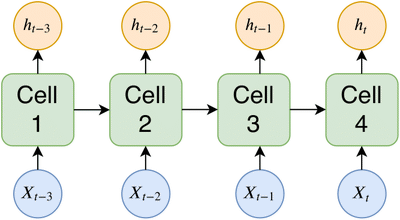
| Typical RNN network structure with RNN cells, here Xt: input time sequence,ht: output time sequence. |
A problem early versions of RNNs suffer from is the vanishing gradient problem, and this led to gradient-based methods having an extremely long learning time in training RNNs. This was because the error gradient, for which gradient-based methods need, vanishes as it gets propagated back through the network. This leads to layers in RNNs, usually the first layers, to stop learning. Therefore when a sequence is long enough, RNNs struggle to propagate information from earlier time steps to later ones. In simpler terms, RNNs suffer from short term memory.
By looking at the figure above, a typical problem early versions of RNNs faced is that cell one would receive a vanishing error gradient because of the decaying error back-flow and, therefore, not be able to propagate the correct information to cell 4. To combat this short term memory, Sepp Hochreiter and Jürgen Schmidhuber introduced a novel type of RNN called long short-term memory (LSTM).
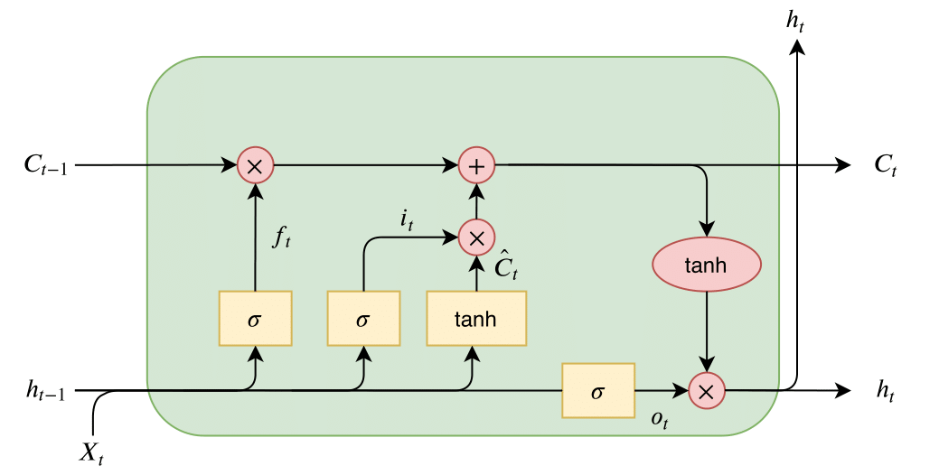
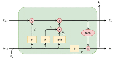
The structure of the LSTM has changed over the years, and here a description of the most common architecture will follow. An LSTM unit is composed of a cell, and within the cell, three gates control the flow of information within the LSTM cell and control the cell state. The three gates are: an input gate, an output gate, and a forget gate. LSTM then chains together these cells, where each cell within the LSTM serves as a memory module.
 |
|---|
| LSTM cell architecture, here Xt: input time step, ht: output, Ct: cell state, ft: forget gate, it: input gate, ot: output gate, Ĉt : internal cell state. Operations inside light red circle are pointwise. |
The three gates, forget, input, and output, can be seen on the figure above as ft, it, and ot, respectively. The gates have a simple intuition behind them:
- The forget gate tells the cell which information to “forget” or throw away from the internal cell state.
- The input gate tells the cell which new information to store in the internal cell state.
- The output gate is then what the cell outputs, this is a filtered version of the internal cell state.

Then the internal cell state is computed as:

The final output from the cell, or ht, is then filtered with the internal cell state as:

Just as with each neural network, weights and biases are connected to each gate. These weight matrices are used in combination with gradient-based optimization to make the LSTM cell learn. Weight matrices and biases can be seen in equations above as Wf, bf, Wi, bi, Wo, bo, and WC, bC respectively.
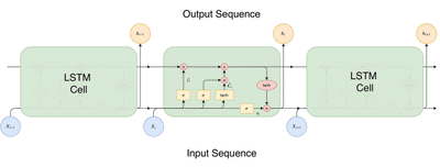
These cells are then chained together, as seen in the figure below; this is what allows the RNN-LSTM network to retain information from past time steps and make time-series predictions. By using the LSTM cell architecture, the network has a way of removing the vanishing gradient problem. This problem hindered older RNN architectures from achieving great time-series predictions.
 |
|---|
| LSTM cells chained together, with input sequence and output sequence shown how used within the network architecture. |
The above architecture is a relatively standard version of an LSTM cell; there are though many variants out there, and researchers constantly tweak and modify the cell architecture to make the LSTM network perform better and more robust for various tasks. An example of this is the LSTM cell architecture introduced in here, where they add peephole connections to each cell gate, which allows each gate to look at the internal cell state Ct-1.
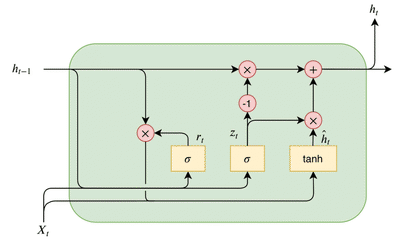
Another prevalent modification of the LSTM is the so-called gated recurrent unit or GRU. The main difference between the GRU and LSTM is that GRU merges the input and forget gates into a single update gate. Moreover, it combines the internal cell state and hidden state. The resulting GRU cell is, therefore, slightly more straightforward than the traditional LSTM. A GRU cell architecture can be seen in the figure below.
 |
|---|
| GRU cell architecture here Xt: input time step, ht: output, rt: reset gate, zt: update gate, ĥt: internal cell state. Operations inside light red circle are pointwise. |
Moreover, in a study found here, which compared eight different LSTM modifications to the traditional LSTM architecture, found that no modification significantly increased performance however it found that changes that simplified the LSTM cell architecture, such as the GRU, reduced the number of parameters and computational cost of the LSTM without significantly decreasing performance.
Parameters in LSTMs
The parameters in a LSTM network are the weight and bias matrices: Wf, bf, Wi, bi, Wo, bo, and WC, bC. Now the size of each weight matrix is: CLSTM * (Fd + CLSTM) where CLSTM stands for the number of cells in the LSTM layer and Fd stands for the dimension of the features. The size of each bias matrix is then of course: CLSTM. Putting this all together we get the total number of parameters in an LSTM network as:

Note this is only for one layer.
Multiply and Accumulation operations in LSTMs
The LSTM inference can be reduced to two matrix-matrix multiplications. The first one can be simplified as:

W is the weight matrix used by the LSTM cell which is composed of Wf, Wi, Wo and WC that are used in equations for the gates and cell state.
Note the dimension of W is (Feature dimension + CLSTM, 4 * CLSTM). Then b is the bias matrix, which is composed of bf, bi, bo and bC.
The final matrix multiplication is then the one needed to compute Ct and ht. Also note that these next multiplications are pointwise. They can be reduced to CLSTM * T MACs, where T is the time series length.
Putting this all together, the total number of MACs in an LSTM layer is:

Thorir Mar Ingolfsson
Postdoctoral Researcher
I develop efficient machine learning systems for biomedical wearables that operate under extreme resource constraints. My work bridges foundation models, neural architecture design, and edge deployment to enable real-time biosignal analysis on microwatt-scale devices.