High-Precision Control and Localisation for Robotic Billiard Shots

In 2018 Joe Warrington started the Automatic Control Lab’s project to build a robotic snooker player capable of challenging a top-ranking human. The project was called DeepGreen, inspired by Deep Blue, the chess computer that famously defeated Garry Kasparov back in 1996. In the spring of 2019 I worked on a research project with Joe that combined robotics, computer vision and a little bit of machine learning.

The project had the title of “High-Precision Control and Localisation for Robotic Billiard Shots” the project aimed at optimally combining the outputs from two cameras to take accurate billiard shots.

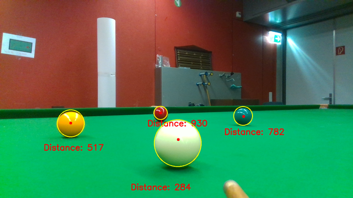
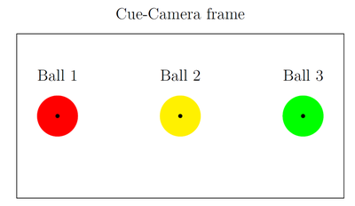
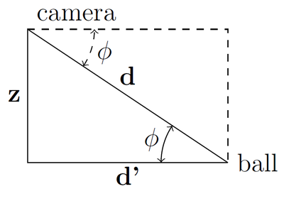
The cue mounted camera, using image processing techniques extracts the $(x,y)$ position in pixel coordinates of each ball as seen in the figure below, the distance to each ball, $d$, is then measured using the built in depth sensor. For being able to accurately estimate the pose of the cue camera we need to have each ball coordinate in a cue camera coordinate system.

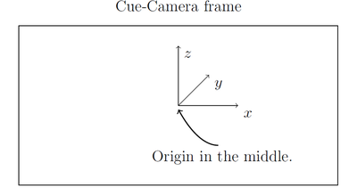
Cue camera coordinate system

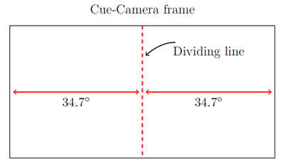
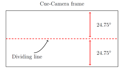
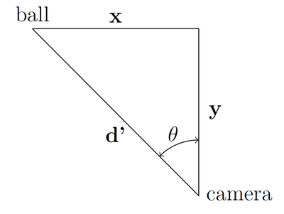
The field of view of the camera is $69.4^{\circ}$ in the horizontal direction and $49.5^{\circ}$ in the vertical direction. We make the assumption that the camera coordinate system is as seen in the figure below. We can then calculate the two angles $\theta$ (horizontal FOV) and $\phi$ (vertical FOV). For $\theta$ we divide the picture into two parts as seen in the figure beow, and we then calculate: \begin{equation} \theta = \frac{|x-640|}{640}\times\frac{69.4^\circ}{2} \label{eqn:theta} \end{equation} Similarly for $\phi$ we get: \begin{equation} \phi = \frac{|y-360|}{360}\times\frac{49.5^\circ}{2} \label{eqn:phi} \end{equation}

Having extracted these two angles we can find the $(x,y,z)$ coordinates of the balls in the camera coordinate system. The $z$-coordinate of the balls is calculated as: \begin{equation} \label{eqn:z_camera} z = -\sin{(\phi)}d \end{equation} As can be seen in the figure above.

The negative sign is because we assume that the camera is always above the balls. For the $(x,y)$ coordinates we calculate the projection of $d$ onto the $x-y$ plane which is given as: \begin{equation} \label{eqn:d_prime} d' = \cos{(\phi)}d \end{equation} The $(x,y)$ coordinate is then calculated as can be seen from figure below.

\begin{equation} \label{eqn:x_y_camera} x = \sin{(\theta)}d', \ \ y = \cos{(\theta)}d' \end{equation} Note if the pixel coordinate of the center of the ball is in the left half plane of the frame then: $$ x = -\sin{(\theta)}d' $$ If we have at least two balls in the camera frame we can estimate the pose of the cue mounted camera.

Orthogonal Procrustes Problem

Now let $$ A_i = (x_i,y_i,0)^T, \ \ i = 1,2,\ldots,N $$ represent the ball position in the world coordinate system. And the corresponding points as seen in the camera coordinate system let them be represented with: $$ B_i = (\tilde x_i,\tilde y_i,\tilde z_i)^T, \ \ i = 1,2,\ldots,N $$ Where $N$ denotes the total number of ball seen. We then should be able to write: $$ A_i = RB_i + T $$ Where $R$ is a 3x3 rotation matrix and $T$ is a 3x1 translation matrix. This kind of problem falls under so called Procrustes analysis, and since we have the necessary condition of $R$ having to be a valid rotation matrix the problem is better known as the Orthogonal Procrustes problem. The name Procrustes refers to a bandit from Greek mythology who made his victims fit his bed by either stretching their limbs or cutting them off. To find $R$ and $T$ we minimize: \begin{equation} \label{eqn:minimization} \min_{R,T} \sum_{i=1}^N \sigma_i^{-2}||A_i - RB_i - T||^2 \end{equation} Where $\sigma_i^{-2}, \ \ i = 1,2,\ldots,N $ accounts for the intrinsic uncertainty of each point pair, $A_i$ and $B_i$. Also define: $$ \boldsymbol{\Sigma_e} = \begin{pmatrix}\sigma_1^{2} & 0 & \dots & 0 \\ 0 & \sigma_2^{2} & \dots & 0 \\ \vdots & \vdots & \ddots & \vdots \\ 0 & 0 & \dots & \sigma_N^{2} \end{pmatrix} $$

$\boldsymbol{\Sigma_e}$ is a diagonal matrix that models the point uncertainty. Now since the true $\boldsymbol{\Sigma_e}$ is not known we can conservatively define the diagonal values of $\boldsymbol{\Sigma_e}$ as follows: $$ \sigma_{i}^{2}=\lambda_{\max }\left(\boldsymbol{\Sigma}_{A_{i}}\right)+\lambda_{\max }\left(\boldsymbol{\Sigma}_{B_{i}}\right) $$ Where $\lambda_{\max}$ denotes the maximum eigenvalue and $$ \boldsymbol{\Sigma}_{A_i} = \begin{pmatrix} \delta \hat{x} & 0 & 0 \\ 0 & \delta \hat{y} & 0 \\ 0 & 0 & \delta \hat{z} \end{pmatrix}, \ \boldsymbol{\Sigma}_{B_i} = \begin{pmatrix} \delta \tilde x & 0 & 0 \\ 0 & \delta \tilde y & 0 \\ 0 & 0 & \delta \tilde z \end{pmatrix} $$ denote the uncertanty matrices of points detected by the overhead camera and cue camera respectively. By taking the derivative with regard to $T$ and setting equal to zero we get: $$ \sum_{i=1}^N\sigma_{i}^{-2}(A_i - RB_i - T) \overset{!}{=} 0
$$ $$ \rightarrow T = \frac{1}{N_{\sigma}}\sum_{i=0}^{N} \sigma_i^{-2}A_i - \frac{R}{N_{\sigma}}\sum_{i=0}^{N} \sigma_i^{-2}B_i $$ or $$ T = \frac{1}{N_\sigma}(\bar{A}\boldsymbol{\Sigma_e^{-1}}\unicode{x1D7D9}- R\bar{B}\boldsymbol{\Sigma_e^{-1}}\unicode{x1D7D9}) $$ or $$ T = \mu_{A} - R \mu_{B} $$ where: $\bar{A} = [A_1,\ldots,A_N]$, $\bar{B} = [B_1,\ldots,B_N]$, $N_\sigma = \sum_{i=1}^{N}\sigma_i^{-2}$, $\unicode{x1D7D9} = [1,1,\ldots,1]^T \in \mathbb{R}^{N} $, $\mu_{A} = \frac{1}{N_\sigma}\bar{A}\boldsymbol{\Sigma_e^{-1}}\unicode{x1D7D9} $ and $\mu_{B} = \frac{1}{N_\sigma}\bar{B}\boldsymbol{\Sigma_e^{-1}}\unicode{x1D7D9}$

We can then rewrite \eqref{eqn:minimization} to be

\begin{align}\label{eqn:minimization_rewritten} \begin{split} & \underset{R}{\text{min}} & & ||A - RB||_F^2\\ & \text{subject to} & \ & R^TR = I_3 \ \ \text{and} \ \det{(R)} = 1 \end{split} \end{align}

where $A = \tilde{A}\boldsymbol{\Sigma_e^{-1/2}}$, $B = \tilde{B}\boldsymbol{\Sigma_e^{-1/2}}$, $\tilde{A} = (A_1 - \mu_A,A_2 - \mu_A,\ldots,A_N - \mu_A)$ and $\tilde{B} = (B_1 - \mu_{B},B_2 - \mu_{B},\ldots,B_N - \mu_{B})$. Now we can write: $$ |A-RB|_{F}^{2}=\operatorname{trace}\left(A^{T} A-2 B^{T}R^{T} A+B^{T} B\right) $$ So the minimization problem \eqref{eqn:minimization_rewritten} can be thought of as maximizing $\operatorname{trace}\left(R B A^{T}\right)$ since $\operatorname{trace}\left(B^{T}R^{T} A\right) = \operatorname{trace}\left(R B A^{T}\right)$ by properties of the trace. Now let $BA^{T} = C$ and then:

$$ \begin{align*} \operatorname{trace}\left(R C\right) & =\operatorname{trace}\left(R U \Sigma V^{T}\right) \\ & =\operatorname{trace}\left(V^{T} R U \Sigma\right) \\ & =\operatorname{trace}(Z \Sigma)\end{align*} $$

Where the singular value decomposition of $C$ is $U \Sigma V^T$ and $\Sigma = \operatorname{diag}(\hat \sigma_1,\hat \sigma_2,\ldots,\hat \sigma_N)$ To maximize $\operatorname{trace}\left(R B A^{T}\right)$ we must look at two cases, when $\operatorname{det}(VU^T) = \pm 1$. Note that the determinant of $VU^T$ can never be anything but $\pm 1$ since $V$ and $U$ are both orthogonal matrices and the product of two orthogonal matrices is also orthogonal.

First we note that $\operatorname{trace}(Z \Sigma) =\sum_{i=1}^{N} z_{i i}\hat{\sigma}_{i} \leq \sum_{i=1}^{N} \ \hat{\sigma}_{i}$ since $Z$ is orthogonal and $z_{i i} \leq 1, \ i = 1,2,\ldots,N$.

If $\operatorname{det}(VU^T) = -1$, then let $D$ be a $N\times N$ orthogonal matrix so that: $\overline{Z}=D^{T} Z D,$ where $\overline{Z}=\left( \begin{array}{cc}{Z_{0}} & {O} \\ {O^{T}} & {-1}\end{array}\right)$ where $Z_{0}$ is the uppermost $N - 1 \times N - 1$ entries of $\overline{Z}$ and $O$ is a vertical column or vector of $N-1$ zeros.

Then let $S=D^{T} \Sigma D = \left( \begin{array}{cc}{S_{0}} & {a} \\ {b^{T}} & {\gamma}\end{array}\right)$ where $S_0$ is the uppermost $N - 1 \times N - 1$ entries of $S$. $a$ and $b$ are vertical columns of $N-1$ entries and $\gamma$ is a scalar.

Then note: $$ \operatorname{trace}(Z \Sigma)=\operatorname{trace}\left(D^{T} Z \Sigma D\right)=\operatorname{trace}\left(D^{T} Z D D^{T} \Sigma D\right)=\operatorname{trace}(\overline{Z}S) = \operatorname{trace}(Z_0S_0) - \gamma $$ We can also write: $$\operatorname{trace}(Z_0S_0) \leq \operatorname{trace}(S_0)$$ where of course: $\operatorname{trace}(S_0) + \gamma = \operatorname{trace}(S) = \operatorname{trace}(\Sigma)$. Now we then have that $\gamma = \sum_{i=1}^{N} d_{iN}^2\hat{\sigma}_i$ so we can write with certainty that $\gamma \geq \hat{\sigma}_N$.

Using all these justifications we can get an upper bound on $\operatorname{trace}(Z \Sigma)$: $$ \operatorname{trace}(Z \Sigma)=\operatorname{trace}\left(Z_{0} S_{0}\right)-\gamma \leq \operatorname{trace}\left(S_{0}\right)-\gamma=\operatorname{trace}(\Sigma)-\gamma-\gamma \leq \sum_{i=1}^{N-1} \hat{\sigma}_{i}-\hat{\sigma}_{N} $$ These are then the two cases we must consider:

• When $\operatorname{det}(VU^T) = 1$ We maximize by choosing $Z = I_N$ so $R = VU^T$ minimizes \eqref{eqn:minimization_rewritten}.
• When $\operatorname{det}(VU^T) = -1$ Then define $\tilde{S} = \operatorname{diag}(1,1,\ldots,-1)$ a $N \times N$ diagonal matrix. And we know that: $$ \operatorname{trace}(R C)=\operatorname{trace}\left(R U \Sigma V^{T}\right)=\operatorname{trace}\left(V^{T} R U \Sigma \right) \leq \sum_{j=1}^{N-1} \hat{\sigma}_{j}-\hat{\sigma}_{N} $$ If we choose $R = V\tilde{S}U^T$, then $R$ is orthogonal and $\operatorname{det}(R) = 1$ and $$ \operatorname{trace}(R C)=\operatorname{trace}\left(V\tilde{S}U^TU\Sigma V^T\right)=\operatorname{trace}\left(V \tilde{S} \Sigma V^T \right) = \operatorname{trace}(\tilde{S}\Sigma) = \sum_{j=1}^{N-1} \hat{\sigma}_{j}-\hat{\sigma}_{N} $$ Thus $R = V\tilde{S}U^T$ minimizes \eqref{eqn:minimization_rewritten}.

Euler Angles

Having estimated the rotation matrix we need to extract the Euler angles since we use them to correct the cue angle. Now let the rotation matrix be: $$ R=\left[ \begin{array}{lll}{R_{11}} & {R_{12}} & {R_{13}} \\ {R_{21}} & {R_{22}} & {R_{23}} \\ {R_{31}} & {R_{32}} & {R_{33}}\end{array}\right] $$ We can then calculate the Euler angles as:

if $R_{31} \neq \pm 1$ $$ \theta \gets -\operatorname{arcsin}\left(R_{31}\right) $$

$$ \psi \gets \operatorname{arctan2} \left(\frac{R_{32}}{\cos{\theta}},\frac{R_{33}}{\cos{\theta}}\right) $$

$$ \phi \gets \operatorname{arctan2} \left(\frac{R_{21}}{\cos{\theta}},\frac{R_{11}}{\cos{\theta}}\right) $$

else $$ \phi \gets 0 $$ and if $R_{31} = -1$ $$ \theta \gets \frac{\pi}{2} $$ $$ \psi \gets \operatorname{arctan2} (R_{12},R_{13}) $$ else $$ \theta \gets -\frac{\pi}{2} $$ $$ \psi \gets \operatorname{arctan2} (-R_{12}-,R_{13}) $$

The most important angle is $\theta$ as that is the one can be thought of as the cue angle on the table.

Uncertainty Estimation

For uncertainty calculations of the cue camera frame of reference ball coordinates. We write: $$ x \pm \delta x , \ \ y \pm \delta y \ \textrm{and} \ d \pm \delta d $$ We can write the distance RMS error as: $$ \text{Distance RMS error (mm)} = \frac{d^2\cdot \text{Subpixel}}{\text{Focal length (pixels)}\cdot \text{Baseline (mm)}} $$ Where $\text{Subpixel} = 0.08$, $\text{Baseline (mm)} = 50$ and $$ \text{Focal length (pixels)} = \frac{1}{2} \frac{\text{Xres (pixels)}}{\tan{\text{HFOV}/2}} = \frac{1}{2} \frac{848}{\tan{45^{\circ}}} $$

Now from \eqref{eqn:theta} and \eqref{eqn:phi} we get that: $$ \delta\theta = \frac{69.4}{1280}\delta x , \ \ \delta\phi = \frac{49.5}{720}\delta y $$ If we have a general function of the form: \begin{equation*} R(X,Y,\ldots) \end{equation*} we can write the uncertainty of that function as: \begin{equation} \label{eqn:general_fcn_uncert} \delta R=\sqrt{\left(\frac{\partial R}{\partial X} \cdot \delta X\right)^{2}+\left(\frac{\partial R}{\partial Y} \cdot \delta Y\right)^{2}+\ldots} \end{equation} Where we assume that variations in $X,Y$ and $Z$ directions are independant. From \eqref{eqn:z_camera} and \eqref{eqn:general_fcn_uncert} we write: $$ \delta \tilde{z} = \sqrt{(-\cos(\phi)\cdot d \cdot \delta \phi)^2+(-\sin{(\phi)}\delta d)^2} $$

Similarly from \eqref{eqn:d_prime} we get: $$ \delta d' = \sqrt{(-\sin(\phi)\cdot d \cdot \delta \phi)^2+(\cos{(\phi)}\delta d)^2} $$ And then from \eqref{eqn:x_y_camera} we get:

\begin{align*} \begin{split} \delta \tilde{x} = \sqrt{(\cos(\theta)\cdot d' \cdot \delta\theta)^2+(\sin{(\theta)}\delta d')^2} \\
\delta \tilde{y} = \sqrt{(-\sin(\theta)\cdot d' \cdot \delta \theta)^2+(\cos{(\theta)}\delta d')^2} \end{split} \end{align*} We then build up the $\boldsymbol{\Sigma}_{B_i}$ matrix for each ball as (where $i = 1,\ldots,N$)

$$ \boldsymbol{\Sigma}_{B_i} = \begin{pmatrix} \delta \tilde x & 0 & 0 \\ 0 & \delta \tilde y & 0 \\ 0 & 0 & \delta \tilde z \end{pmatrix} $$

Then we can build up the $\boldsymbol{\Sigma}_{A_i}$ matrix for each ball as (from overhead camera uncertainty):

$$ \boldsymbol{\Sigma}_{A_i} = \begin{pmatrix} 3 & 0 & 0 \\ 0 & 3 & 0 \\ 0 & 0 & 0 \end{pmatrix} $$

Note that the error on the z-value in $\boldsymbol{\Sigma}_{A_i}$ is 0 since we know that each ball is on the table and not hovering over it or under it.

With each new measurement our belief of the rotation and translation is updated according to the following: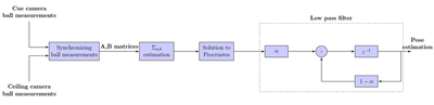

Where we implement a low pass filter to filter out high frequency changes in rotation and translation that might influence the pose estimation negatively.

Shot-Taking Algorithm

The robot arm moves to a starting position which are calculated from the overhead camera, this starting position and angle of shot is very crude and often results in the cue striking the ball at an undesirable position. We then implemented a feedback loop that adjusts the cue position based on the pose estimation presented in the figure above

Shot-angle calculation

To calculate the angle that the cue should be pointing in we use the ghost ball method. By drawing a line from the middle of the pocket through the center of the target ball one can see where the cue ball should strike the target ball as illustrated in the figure below.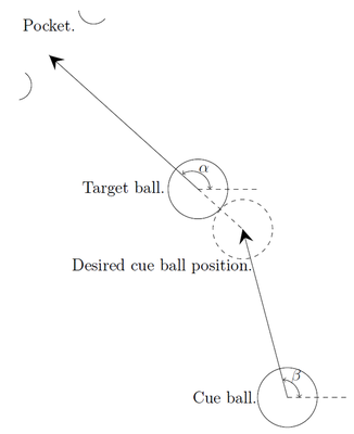

Let the $(x,y)$ positions of the pocket, target ball, cue ball be denoted by $(x_p,y_p), \ (x_t,y_t), \ (x_c,y_c)$ respectively and let the position of the “ghost ball” or desired cue ball position be denoted by $(x_g,y_g)$. We can then calculate: $$ \alpha = \operatorname{arctan2} (y_p - y_t, x_p - x_t) $$ The desired cue ball position can then be calculated as: $$ (x_g, y_g) = (x_t - \cos{\alpha} \cdot 52.5, y_t - \sin{\alpha} \cdot 52.5) $$ Where $52.5$ is the diameter of a snooker ball and the shot angle is then calculated as: \begin{equation} \label{eqn:shot_angle} \beta = \operatorname{arctan2} (y_g - y_c,x_g - x_c) \end{equation}

Shot Difficulty Metric

Each shot the robot tries to make has a difficulty metric which is defined as: \begin{equation*} \textbf{difficulty} = \frac{d_1\cdot d_2}{\cos{\tilde{\theta}}} \end{equation*} Where $d_1$ is the distance between cue ball and target ball, $d_2$ is the distance between target ball and pocket. $\tilde{\theta}$ is the cut angle. As depicted on the figure below.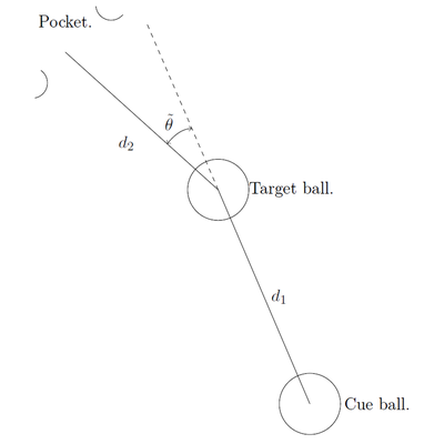

Feedback correction

Two approaches to the feedback correction were implemented and tested, location based and image based.

Location based feedback correction

In the location based feedback approach we had a fixed $(x,y)$ position on the snooker table that we wanted the cue to be in. By reading of the first two lines in the translation matrix that we get from the pose estimation we were then able to correct the cue position until a threshold was met. At the same time the shot angle \eqref{eqn:shot_angle} was calculated and the cue rotated in the correct direction. This method quickly proved to be too noisy to use, and resulted in the cue striking the ball in very undesirable locations or simply not striking the cue ball at all. We then moved on to the next method to implement the feedback correction.

Image based feedback correction

Since the location based feedback correction was not robust enough for the high precision task of striking the cue ball in a precise location, we used a different approach to correcting the $(x,y)$ position of the cue. By testing we saw that the ball striking was best if the cue camera was approximately $261$ millimeters from the cue ball. And the cue struck the cue ball dead center if it was at a fixed point $(\tilde{x}, \tilde{y})$ in the cue camera frame as is illustrated in the figure below. As well as we used the Procrustes solution for the rotation matrix to rotate the cue to the correct shot angle.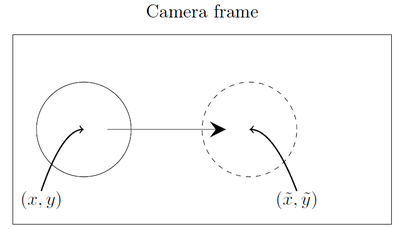

So the procedure went as is shown in the figure below.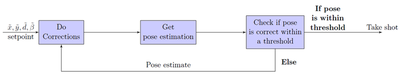

In practice there is also lag implemented to allow the pose estimate to settle after each feedback correction.

Video of Performance

Putting all this math together (with a lot of programming) we can see the following performance: